


Articles
TI accelerates the shift toward autonomous vehicles with expanded automotive portfolio
New analog and embedded processing technologies from TI enable automakers to deliver smarter, safer and more connected driving experiences across their entire vehicle fleet
Articles
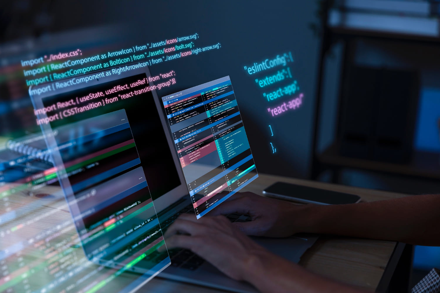
Monitor Tableau Cloud Deployments of Any Size with the Platform Data API
Tableau puts self-service visual analytics within reach of everyone, from small businesses with just a few licenses to massive enterprises deploying it across their entire
Articles
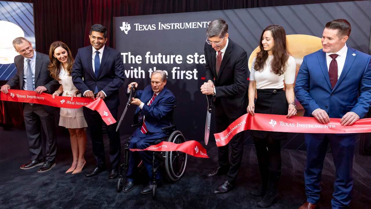
Texas Instruments begins production at its newest 300mm semiconductor manufacturing facility in Sherman, Texas
State-of-the-art wafer fab will produce tens of millions of chips daily that go into nearly every electronic device